QGIS Tutorial II: from data to map – preparing data visualisation

In this tutorial I would like to show you, how to create a topographic map and analyse topographical data using freely available SRTM data and QGIS including some data manipulation. This is part one explaining how to get data, remove missing values, explore the relief and changing the color representation of a TIF file obtained by the USGS.

• Downloading SRTM data and installing GRASS plugin
• Prepare the data for the processing in GRASS and remove NoData values
• process a shaded relief in GRASS and prepare for map creation

objective

<

p align=”justify”>A basis for several analytical steps is the surface of the earth. We differentiate therefore surface and the elevation as buidlings, tree cover and other elements create their own surface which is higher than earths elevation. We will visualize a near-elevation model obtained by the Shuttle Radar Topographic Mission in a map.

what do you need

• Quantum GIS (examples shown in QGIS 1.8) with GRASS support
• SRTM data

time effort

approx. 30 minutes

step 1 – download data, install plugin

We need to download some data from the USGS. In most cases I use landcover.org. Just search for the desired location (I often use path and rows which can be calculated and are better to remember) and use SRTM WRS-2 Tiles:

I have used the filled-finished B version of my area. You can download the example dataset directly as well (copyright University of Maryland, but what about a CC-license?!).

On the QGIS site make sure, that you have installed QGIS properly and you have the GRASS plugin enabled:

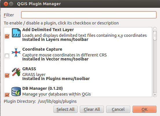
You can find some hints on how to enable GRASS for QGIS on Mac. On Windows machines it should be easy due to the standalone installer.

preparing data

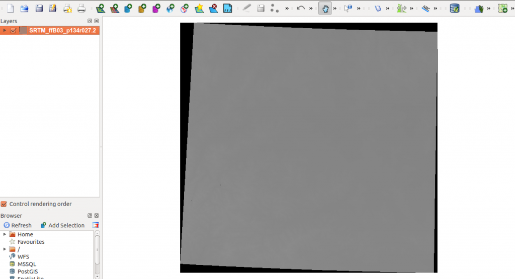
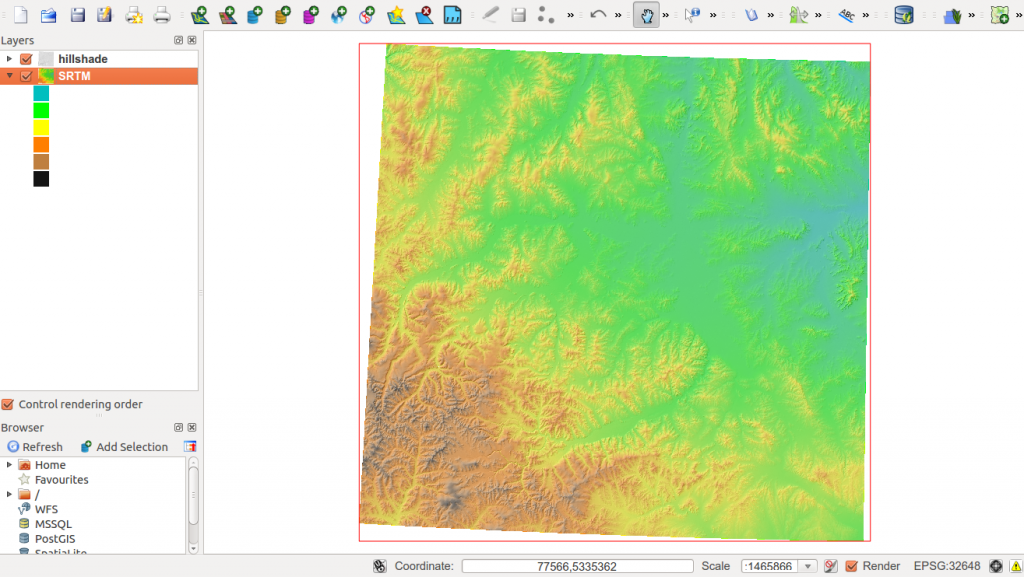
After unzipping the data we should start with the preparation of the data in QGIS / GRASS. You may ask, why I’m not using QGIS only for this topographic map as it has a tool called “Terrain Analysis Plugin” for this. Short answer: data quality. As you have added the raster to your project you may see something like this:

<

p align=”justify”>Using the info tool you will see, that the black areas in and outside of the real scene are pixels with the value “-32768” which is the smallest possible value in the unsigned integer 16 value range which is [-32768 , 32768 ]. As it is possible to display 256 different types of grey, all important values can only be shown in prob. ten types of grey. So we need to define this record for a missing value as “null” or “NoData”. If you won’t do that and you will calculate slope you will get broad plaines around your area of interest and you may forget everything that starts with word stats…

Now GRASS comes into play. GRASS has a function called r.null.val which converts numbers to “null”-values. But using GRASS is a pain in the arse first time: You need to define a working area beforehand.

• Go to Plugins->GRASS->New Mapset
• define a folder to store te results and your data
• create a location (in my case Mongolia)
• now define the projection for your GRASS project. I love the UTM zones so I choose EPSG:32648 (WGS 84 UTM Zone 48 N)
• define an area that is of interest to work at: every process is spatially “limited” to that region by default. You may choose Mongolia, if you’re not sure about the coordinates
• choose a mapset name that is user specific and defines somehow your own project

We are nearly ready to clean up our data but as a last step we need to import our SRTM image into the GRASS project. Use Plugins->GRASS->Open GRASS tools and use the Modules List to find the function r.in.gdal. Now choose your SRTM tif-file for the import and choose a name for the imported dataset:

Add your raster to your workplace by Plugins->GRASS->Add GRASS Raster Layer.
The last preparational step is to change the value “-32768” to “noData”. Therefore search the function r.null.val in the Modules List as we have done it for the import. select your dataset (SRTM for me) and type the value “-32768” as the value that represents “noData”. Don’t forget to restrict the working area to the tif itself by enabling the “region button”: . Now enjoy the first special moment:

contrast enhancement due to image cleaning

map: data processing

For the map it is better to have a good visual effect and create some easy consumable information. So an idea is to create a pseudo-3D effect to represent height information. This is called shaded relief and gives you an idea about the shape of mountains, valleys and slopes.
Search for the shaded relief module in the GRASS toolbox and select the processed SRTM dataset as input (don’t forget to restrict the region as done above as well) and a name for your output. Please change parameters to azimuth “315” and altitude “45” to increase the visual effect, press run and add the output to the map afterwards. If you see some failure stating that QGIS was unable to open the raster, this ressource on gis.stackexchange solved the problem in my case. At the end open the properties of the shaded relief layer by right click on the layer name and change the global transparency to 50% or a value of your choice. Make sure that the shaded relief layer is above the SRTM layer.

difference between a shaded and non-shaded relief

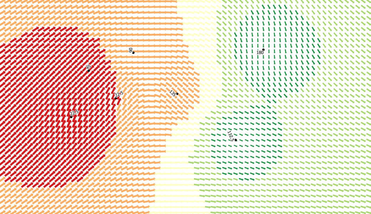
Now you should ask yourself: Where do I get colours for my heights? There is another module in GRASS which creates a color table using some rules. So use the module r.colors.table to create a color table of your choice:

Last but not least prepare the layer for map creation: change the title in the General tab of the SRTM layer as it serves as a legend item and change the label of classes in the colormap tab in the properties.

Map creation

See this in following part 2.