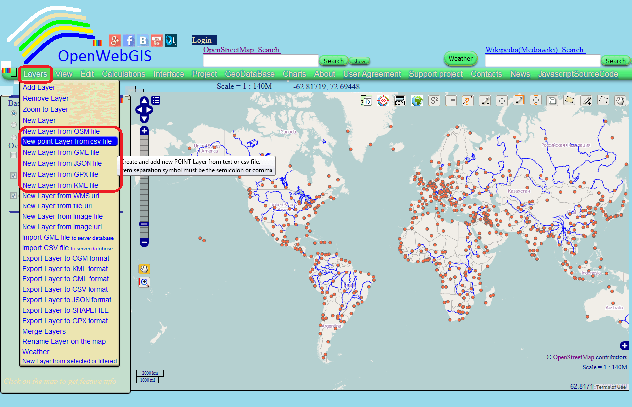
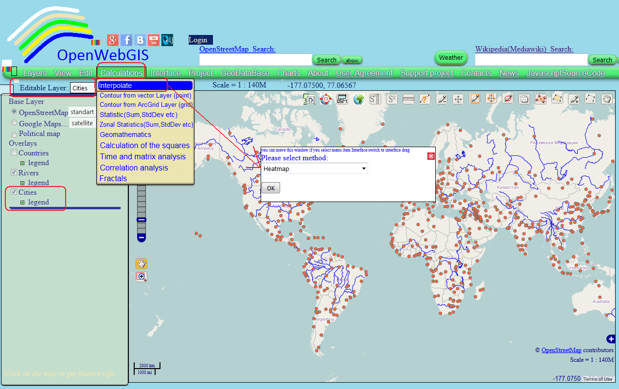
In this article we consider the creation of Heatmap and Interpolation with the help of OpenWebGIS interface. In the next article it is planned to describe its technical implementation using JavaScript, OpenLayers 2.x and canvas element (as part of HTML5 technology). Recently, in an article “Some new (June 2015) features and functions in OpenWebGIS” it has been announced to revise the interpolation module completely. This promise has been kept, and at the moment in OpenWebGIS you can build a heatmap and make interpolation by the method of Inverse Distance Weighting (IDW). It is planned to add (if it is possible) one of the varieties of Kriging interpolation. You can do it with any of your point data, even without downloading them to the server of OpenWebGIS and without registration. You just need to add to the map the data from your file (csv, gml, geoJSON, kml, gpx, osm) with the help of the corresponding menu items “Layers” (see Figure 1).
Later in the article we will consider the work of Heatmap functions and Interpolation based on a point layer “Cities” which is the data about cities (certainly about not all of them) and a population of them around the world. This layer is added to the map of OpenWebGIS by default. So, first of all you need to select the name of the layer with which we will work in the list of “Editable Layer” and click on the menu item “Calculations-> Interpolation” and a pop-up window will appear to select the heatmap or interpolation method (see Figure 2).
Here we consider only “Heatmap” and “Inverse Distance Weighting (IDW)”. If you select methods of “Heatmap (additional)” or “Barnes Surface” to interpolate the point Layer uploaded in OpenWebGIS server, then interpolation results will be shown in WMS Layer. If you interpolate the point Layer which is not uploaded in OpenWebGIS server, but created from csv, gml, kml and etc files, then interpolation (with methods ‘Heatmap (additional)’ or ‘Barnes Surface’) results will be shown in point vector Layer. Let’s start with the heatmap creation. After selecting the corresponding item in the list, the pop-up window will appear with the heatmap parameters. The user can specify any color gradient for the heatmap (you simply click on the corresponding rectangle with the color and choose the desired color (see Figure 3), blur and radius is specified in pixels.
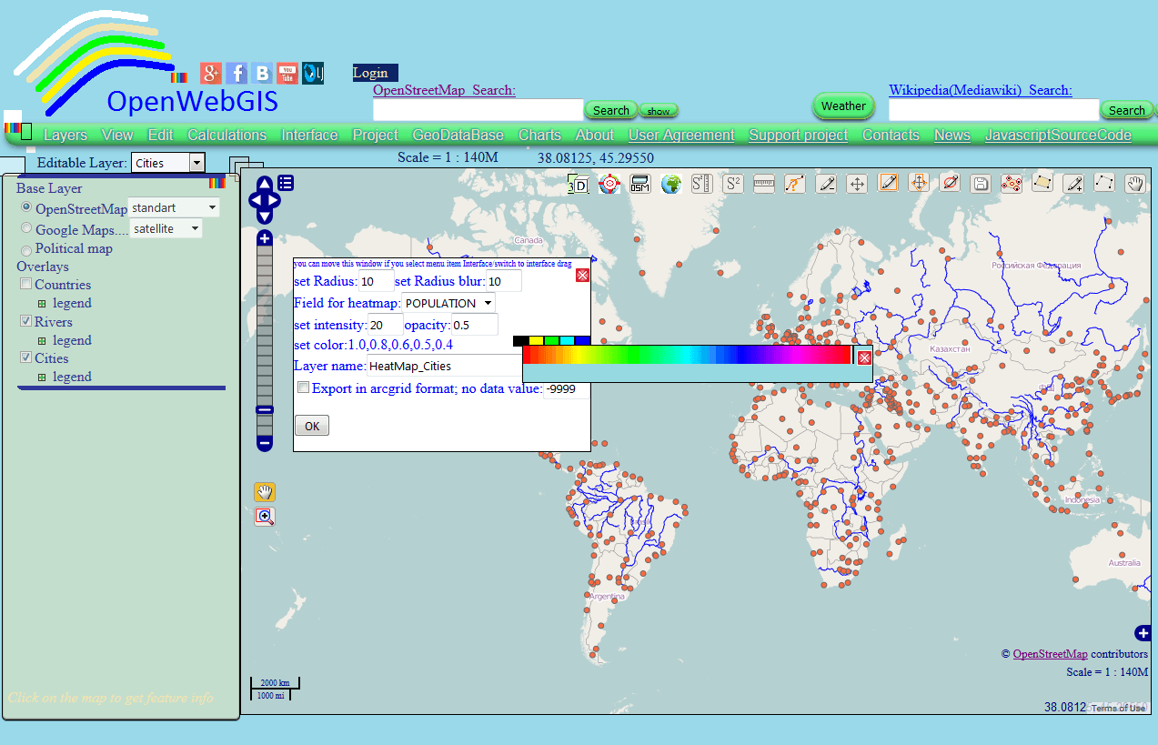
Intensity parameter (intens) is used if you have specified “Field for heatmap” and is put into calculations that in javascript looks like this:
var xfeat = (parseFloat (Layer.features [i].attributes[field])*100)/max;
var count = Math.abs(Math.round(xfeat)/intens);
if (count==0) {count=1;}
for (var t=0; t<count; t ++)
{ctx.drawImage (brushCanvas, x - r, y - r);}
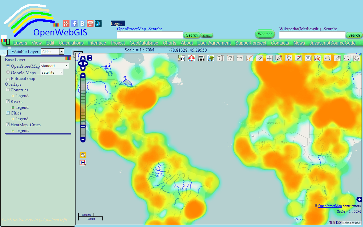
where max is the maximum value of the selected field in the point layer on the base of which we build a heatmap (in this case – the number of population in the city), ctx – context of canvas, r – brush size. In short, intensity depends on the value of the selected field, the number of times will be calculated that the brush will be applied at this point (pixel), if it is done many times then it will be more red (or any other color that you have specified for the maximum value). More information about the program code will be given in the next article. You can download the javascript code from the main menu of OpenWebGIS. As a result, after setting all the desired parameters, press Ok, and you will see the result shown in Figure 4.
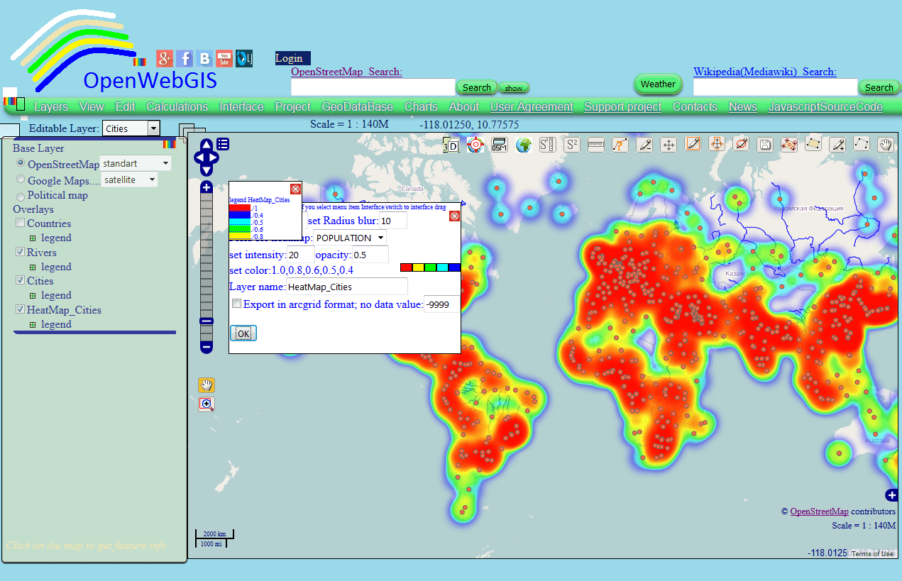
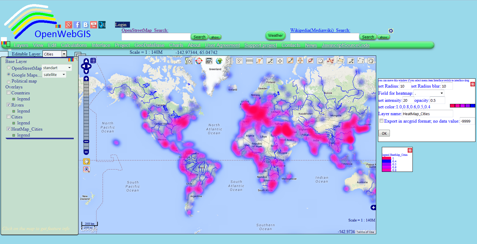
The window with the heatmap parameters can be closed or moved to any convenient place for us if you select menu item “Interface -> Switch to interface drag”, and then click on it to fix a pop-up window. See the result with other settings and a basic map on Figure 5. The result map itself can be seen in the link.
Now we will describe the principle of the IDW interpolation method using an interface of OpenWebGIS. After selecting the appropriate item in the list of methods (as described above) you will see a pop-up window as shown in Figure 6.
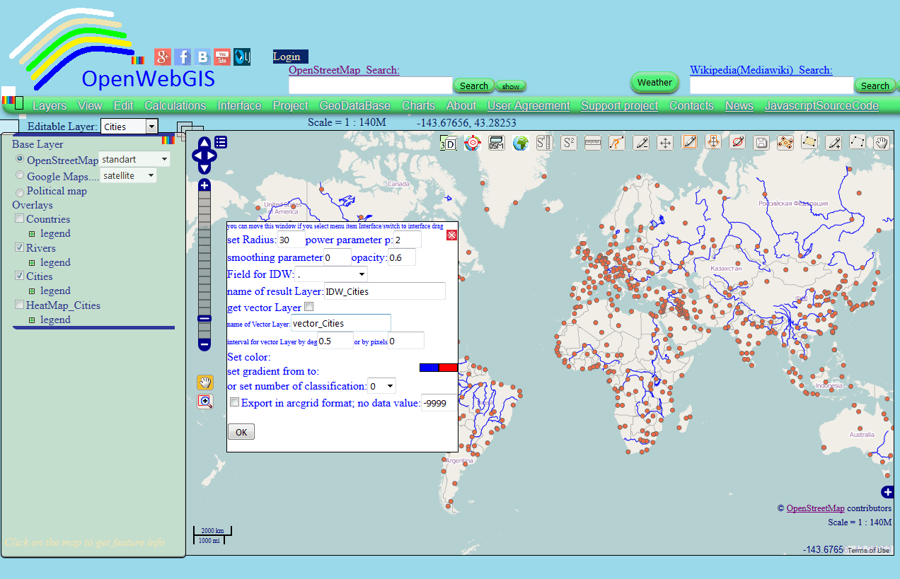
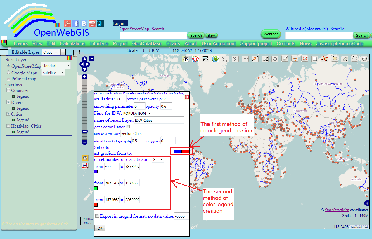
In this window, it is necessary to select the field which will be used for interpolation. You can set a color legend of the interpolation result in two different ways, either using a gradient of 2 colors, or settting the color for each interval of values of the selected field (see Figure 7).
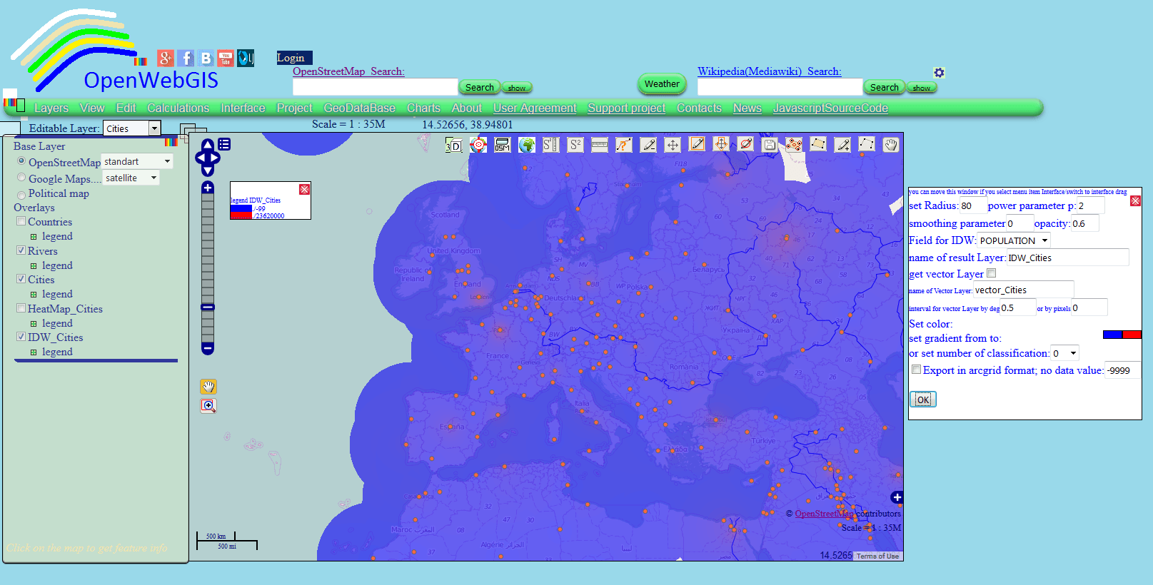
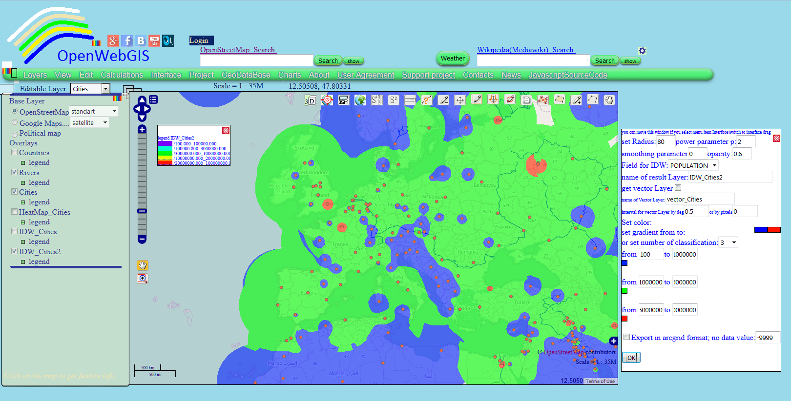
It is important to understand that during the calculation of the interpolation, multiple calculation of distances between points (pixels) occurs , and so it is a resource-intensive process for the browser and the CPU, so you will need to wait for a while for the results depending on the parameters you set. The radius value strongly influences the speed of calculation. The more it is, the longer the calculation is. The interpolation results of the number of population according to the color legend created by a gradient is shown in Figure 8. And the color legend created by specifying the colors for the three intervals is shown in Figure 9.
With IDW interpolation settings window you can make a regular vector grid from your data, if you activate the option “get vector Layer”. The grid can be done through a certain inteval of degrees or pixels. In Figure 10 the grid is shown that was got through 10 pixels.
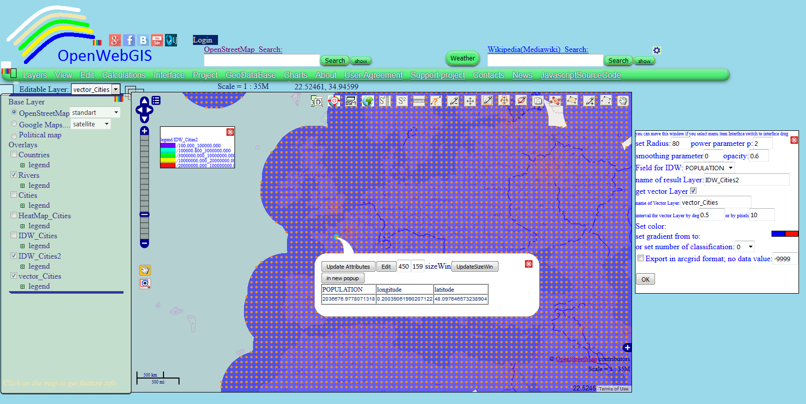
After zoom in zoom out of the map, layers with heatmap and interpolation are automatically recalculated and redrawn. Both in the creation of heatmap and interpolation, you can export the results to ArcGrid ASCII if you activate the option “Export in arcgrid format”.
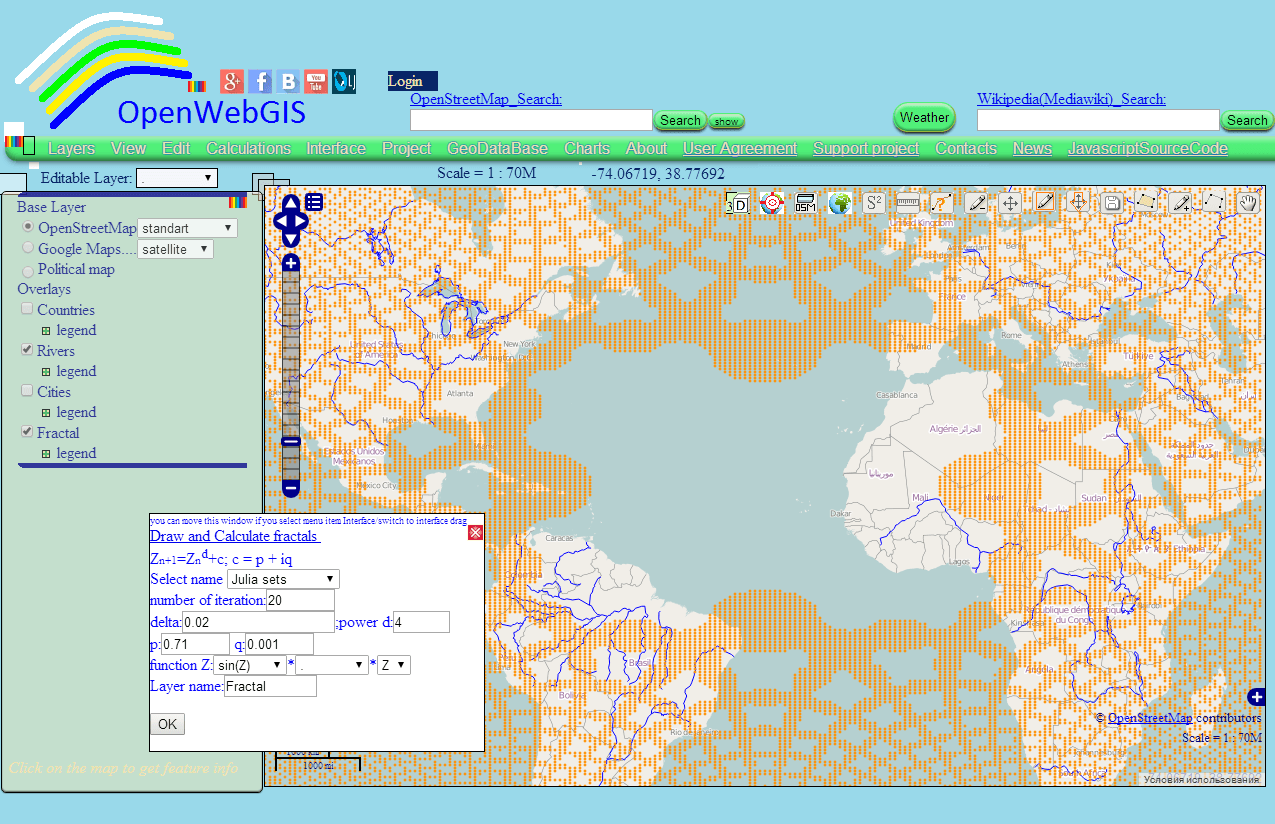
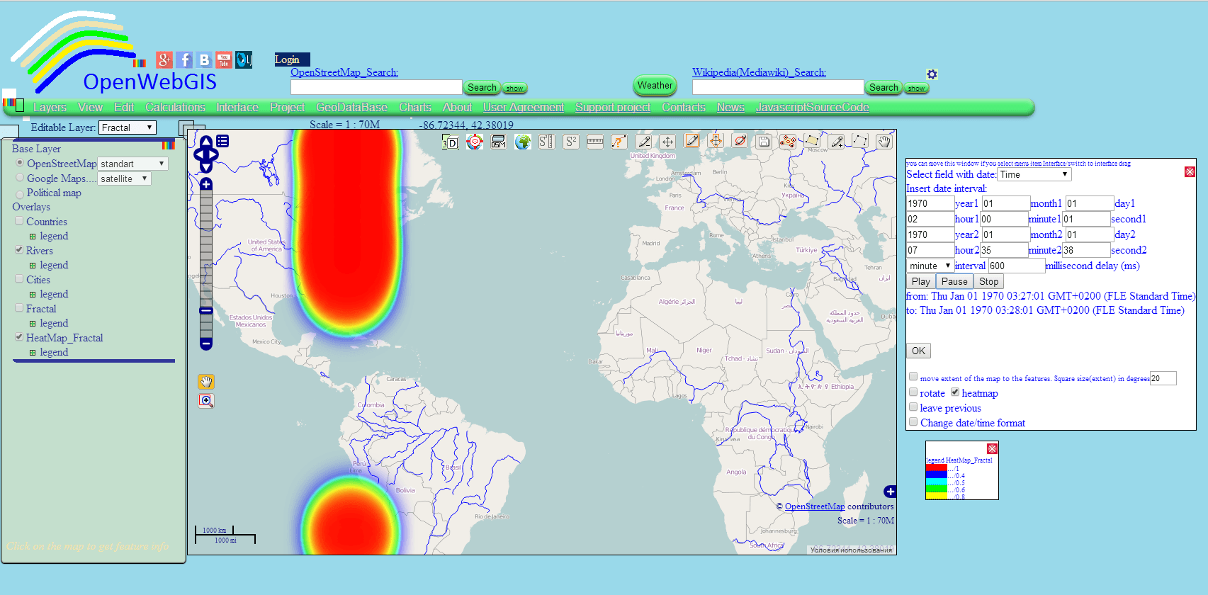
In addition to static heatmap it is often necessary to see a dynamic change in data over time in the form of a heatmap. This ability is present in many online GIS and it is now available in OpenWebGIS. For experimenting with it, let us create an abstract set of data via the menu item “Calculations-> Fractals”. About the creation of fractals you can read more in the article “Create fractals on the map by using OpenWebGIS“. Create a fractal with the parameters indicated in Figure 11.
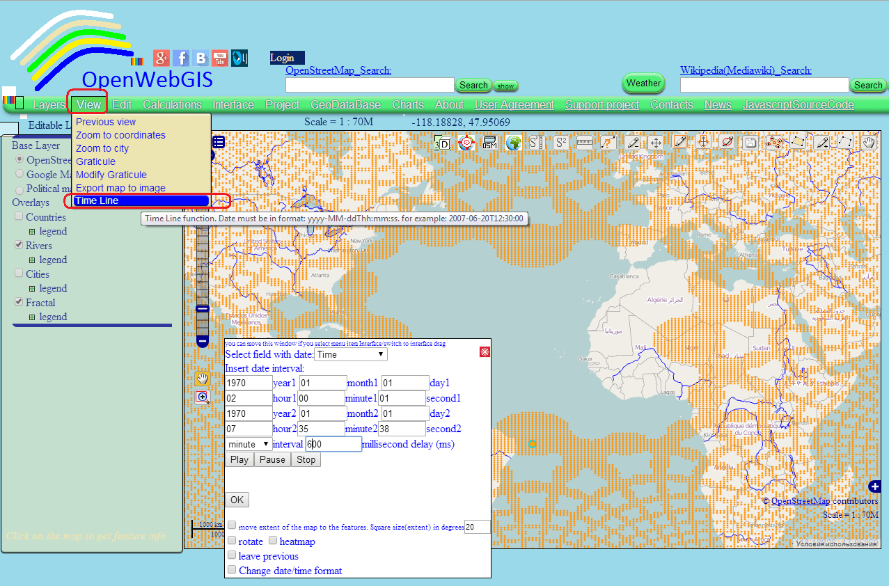
Note – This fractal is built for a long time, probably you will have to wait up to 1 minute. The name of the resulting layer “Fractal” you choose in the list of “Editable Layer” and click on the menu item “View-> Time Line”, specify the parameters in the window as it is shown in Figure 12, then activate the option “heatmap”.
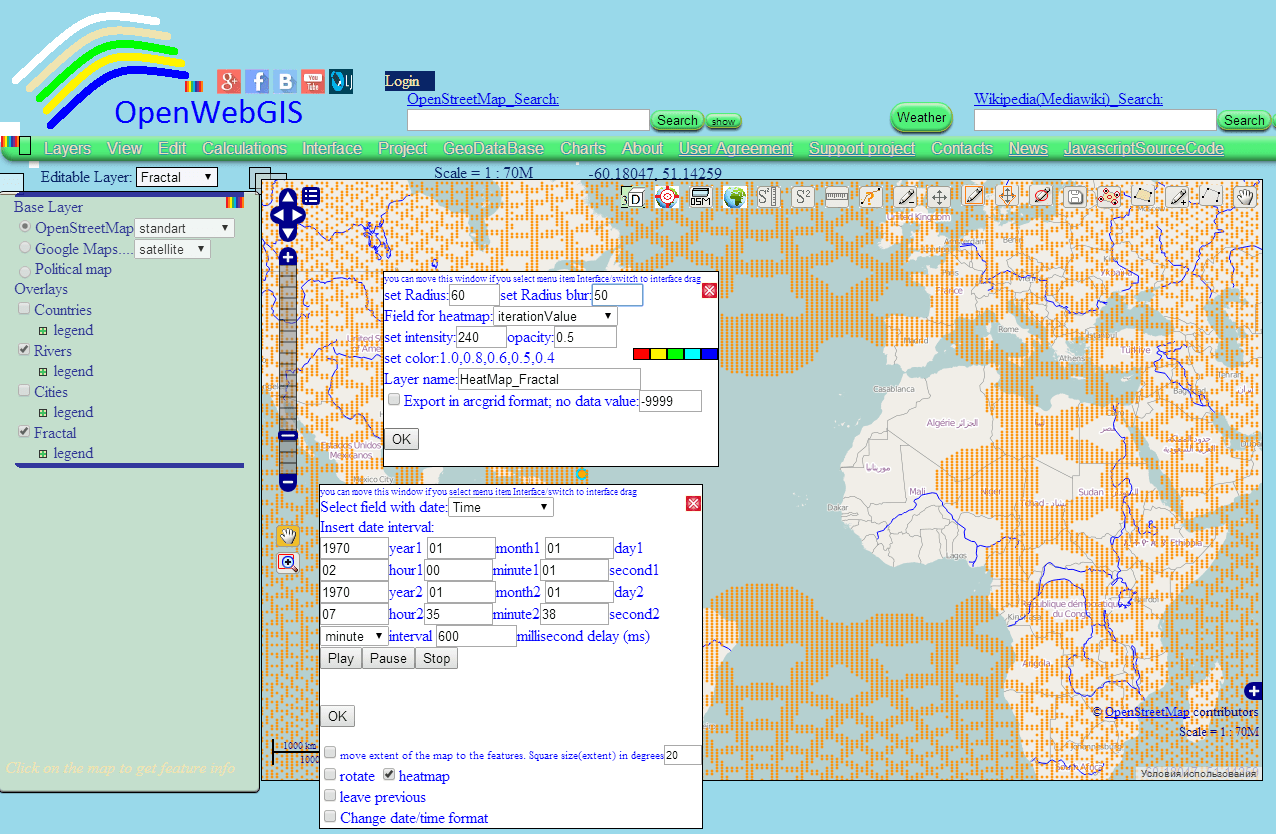
After this a pop-up window with the options of creating heatmap will appear, set the values as it is shown in Figure 13, then click “Ok”, and then “Play” and you’ll see something similar to what is shown in Figure 14. The ready animated map you can see at this link
Read more about using “Time Line” function in the article: “Embedding animated maps of OpenWebGIS in your sites“. It is important to remember that: In opened pop-up window “Time Line” you must select the field (attribute) with date. Dates/times in the field with date must be in format ISO8601: yyyy-mm-ddThh:mm:ss (for example: “1951-08-17T18:00:00”).
Now there is a possibility to vizualise OpenWebGIS data on 3D Globe. So you can visualise a heatmap also on the 3D Globe. See the result in Figure 16.
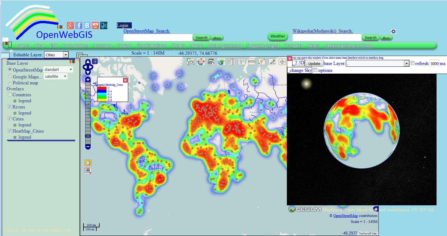
For more information about creating a 3D view, you can read for example in these articles: Creating a 3D city model in OpenWebGIS (Extruding 2D polygons to 3D) , Creating 3D track of International Space Station with the help of OpenWebGIS, Transform Earth Globe to Mars, Venus, Jupiter, Mercury and Sun. Using OpenWebGIS in astrogeology, OpenWebGIS: Changing the sky (background) around the Earth in 3D View, OpenWebGIS is now in 3D! or see video: 3D modelling of buildings on the OpenWebGIS map based on OpenStreetMap
The entire process of creating the heatmap you can see in this video: